How good are strategic intelligence forecasts?

Screen Shot 2014-09-25 at 10.33.10 PM

This is a freshly pressed post that appeared September 25 (today) in Policy Options magazine. In it, I describe how the 6-year intelligence forecasting accuracy study that Alan Barnes and I undertook developed. A detailed description of that study was published in a recent PNAS article that was subsequently summarized in this piece in The Economist. Note that the Economist referred to a 76% accuracy rate. That’s wrong. It was 94%, as indicated in the PNAS paper and today’s post. The 76% figure was actually the adjusted normalized discrimination index value, which is akin to an adjusted eta-squared value — namely, the proportion of variance in the outcomes explained by the intelligence forecasts.

The Futility of Significance (Statistical, that is)

A wonderful surprise arrived in my gmail inbox this morning. A message from Neil Thomason, a dear colleague of mine, who sends me interesting things to read from time to time. It’s not that much of the time the things Neil sends me aren’t that interesting. It’s just that the interesting things he does send me only come from time to time.

Last time he sent me something, it was this Many Labs paper on replications available at the Open Science Forum. Clearly, Neil was impressed. Ten of 13 classic effects were well replicated, one was so-so, and two were not replicated. Neil must have thought I was having a bad day when I clearly was not sharing in the joy. The main reason for that has to do with the fact that effects and explanations of effects are seldom properly decoupled. As a result, a replication of a classic effect is often communicated as a replication of the explanation of the effect. But of course an effect can be highly replicable yet explained in an entirely improper manner. I believe that the authors of the Many Labs paper fell into that trap of not adequately separating the effects they replicated from the standard interpretations given to them. I went on in my reply at some length about the inherent dangers of doing so (and I should blog about this in a separate post at some point in the future).

I confess that I was disappointed not to get a reply from Neil since I thought my comments posed a thoughtful reply to his exuberant reaction. I thought those comments would spark a lively discussion of the issue, perhaps leading us toward some sound principles to guide similar future endeavours. Neil is after all a philosopher of science.

At any rate, nearly 3 months later, this morning, I got a message from him. Just this link to a blog post by Matthew Hankins entitled “Still Not Significant.” I really enjoyed the post, which deals with the many creative ways researchers find to describe their results when their statistical significance values are at or greater than the magical p < 0.05 level. I encourage you to read the post, but just in case you’re too busy or lazy to do so, I’ve reproduced the list of circumlocutory expressions quoted there. I warn you, the list is long, but also entertaining:

(barely) not statistically significant (p=0.052)
a barely detectable statistically significant difference (p=0.073)
a borderline significant trend (p=0.09)
a certain trend toward significance (p=0.08)
a clear tendency to significance (p=0.052)
a clear trend (p<0.09)
a clear, strong trend (p=0.09)
a considerable trend toward significance (p=0.069)
a decreasing trend (p=0.09)
a definite trend (p=0.08)
a distinct trend toward significance (p=0.07)
a favorable trend (p=0.09)
a favourable statistical trend (p=0.09)
a little significant (p<0.1)
a margin at the edge of significance (p=0.0608)
a marginal trend (p=0.09)
a marginal trend toward significance (p=0.052)
a marked trend (p=0.07)
a mild trend (p<0.09)
a moderate trend toward significance (p=0.068)
a near-significant trend (p=0.07)
a negative trend (p=0.09)
a nonsignificant trend (p<0.1)
a nonsignificant trend toward significance (p=0.1)
a notable trend (p<0.1)
a numerical increasing trend (p=0.09)
a numerical trend (p=0.09)
a positive trend (p=0.09)
a possible trend (p=0.09)
a possible trend toward significance (p=0.052)
a pronounced trend (p=0.09)
a reliable trend (p=0.058)
a robust trend toward significance (p=0.0503)
a significant trend (p=0.09)
a slight slide towards significance (p<0.20)
a slight tendency toward significance(p<0.08)
a slight trend (p<0.09)
a slight trend toward significance (p=0.098)
a slightly increasing trend (p=0.09)
a small trend (p=0.09)
a statistical trend (p=0.09)
a statistical trend toward significance (p=0.09)
a strong tendency towards statistical significance (p=0.051)
a strong trend (p=0.077)
a strong trend toward significance (p=0.08)
a substantial trend toward significance (p=0.068)
a suggestive trend (p=0.06)
a trend close to significance (p=0.08)
a trend significance level (p=0.08)
a trend that approached significance (p<0.06)
a very slight trend toward significance (p=0.20)
a weak trend (p=0.09)
a weak trend toward significance (p=0.12)
a worrying trend (p=0.07)
all but significant (p=0.055)
almost achieved significance (p=0-065)
almost approached significance (p=0.065)
almost attained significance (p<0.06)
almost became significant (p=0.06)
almost but not quite significant (p=0.06)
almost clinically significant (p<0.10)
almost insignificant (p>0.065)
almost marginally significant (p>0.05)
almost non-significant (p=0.083)
almost reached statistical significance (p=0.06)
almost significant (p=0.06)
almost significant tendency (p=0.06)
almost statistically significant (p=0.06)
an adverse trend (p=0.10)
an apparent trend (p=0.286)
an associative trend (p=0.09)
an elevated trend (p<0.05)
an encouraging trend (p<0.1)
an established trend (p<0.10)
an evident trend (p=0.13)
an expected trend (p=0.08)
an important trend (p=0.066)
an increasing trend (p<0.09)
an interesting trend (p=0.1)
an inverse trend toward significance (p=0.06)
an observed trend (p=0.06)
an obvious trend (p=0.06)
an overall trend (p=0.2)
an unexpected trend (p=0.09)
an unexplained trend (p=0.09)
an unfavorable trend (p<0.10)
appeared to be marginally significant (p<0.10)
approached acceptable levels of statistical significance (p=0.054)
approached but did not quite achieve significance (p>0.05)
approached but fell short of significance (p=0.07)
approached conventional levels of significance (p<0.10)
approached near significance (p=0.06)
approached our criterion of significance (p>0.08)
approached significant (p=0.11)
approached the borderline of significance (p=0.07)
approached the level of significance (p=0.09)
approached trend levels of significance (p0.05)
approached, but did reach, significance (p=0.065)
approaches but fails to achieve a customary level of statistical significance (p=0.154)
approaches statistical significance (p>0.06)
approaching a level of significance (p=0.089)
approaching an acceptable significance level (p=0.056)
approaching borderline significance (p=0.08)
approaching borderline statistical significance (p=0.07)
approaching but not reaching significance (p=0.53)
approaching clinical significance (p=0.07)
approaching close to significance (p<0.1)
approaching conventional significance levels (p=0.06)
approaching conventional statistical significance (p=0.06)
approaching formal significance (p=0.1052)
approaching independent prognostic significance (p=0.08)
approaching marginal levels of significance p<0.107)
approaching marginal significance (p=0.064)
approaching more closely significance (p=0.06)
approaching our preset significance level (p=0.076)
approaching prognostic significance (p=0.052)
approaching significance (p=0.09)
approaching the traditional significance level (p=0.06)
approaching to statistical significance (p=0.075)
approaching, although not reaching, significance (p=0.08)
approaching, but not reaching, significance (p<0.09)
approximately significant (p=0.053)
approximating significance (p=0.09)
arguably significant (p=0.07)
as good as significant (p=0.0502)
at the brink of significance (p=0.06)
at the cusp of significance (p=0.06)
at the edge of significance (p=0.055)
at the limit of significance (p=0.054)
at the limits of significance (p=0.053)
at the margin of significance (p=0.056)
at the margin of statistical significance (p<0.07)
at the verge of significance (p=0.058)
at the very edge of significance (p=0.053)
barely below the level of significance (p=0.06)
barely escaped statistical significance (p=0.07)
barely escapes being statistically significant at the 5% risk level (0.1>p>0.05)
barely failed to attain statistical significance (p=0.067)
barely fails to attain statistical significance at conventional levels (p<0.10
barely insignificant (p=0.075)
barely missed statistical significance (p=0.051)
barely missed the commonly acceptable significance level (p<0.053)
barely outside the range of significance (p=0.06)
barely significant (p=0.07)
below (but verging on) the statistical significant level (p>0.05)
better trends of improvement (p=0.056)
bordered on a statistically significant value (p=0.06)
bordered on being significant (p>0.07)
bordered on being statistically significant (p=0.0502)
bordered on but was not less than the accepted level of significance (p>0.05)
bordered on significant (p=0.09)
borderline conventional significance (p=0.051)
borderline level of statistical significance (p=0.053)
borderline significant (p=0.09)
borderline significant trends (p=0.099)
close to a marginally significant level (p=0.06)
close to being significant (p=0.06)
close to being statistically significant (p=0.055)
close to borderline significance (p=0.072)
close to the boundary of significance (p=0.06)
close to the level of significance (p=0.07)
close to the limit of significance (p=0.17)
close to the margin of significance (p=0.055)
close to the margin of statistical significance (p=0.075)
closely approaches the brink of significance (p=0.07)
closely approaches the statistical significance (p=0.0669)
closely approximating significance (p>0.05)
closely not significant (p=0.06)
closely significant (p=0.058)
close-to-significant (p=0.09)
did not achieve conventional threshold levels of statistical significance (p=0.08)
did not exceed the conventional level of statistical significance (p<0.08)
did not quite achieve acceptable levels of statistical significance (p=0.054)
did not quite achieve significance (p=0.076)
did not quite achieve the conventional levels of significance (p=0.052)
did not quite achieve the threshold for statistical significance (p=0.08)
did not quite attain conventional levels of significance (p=0.07)
did not quite reach a statistically significant level (p=0.108)
did not quite reach conventional levels of statistical significance (p=0.079)
did not quite reach statistical significance (p=0.063)
did not reach the traditional level of significance (p=0.10)
did not reach the usually accepted level of clinical significance (p=0.07)
difference was apparent (p=0.07)
direction heading towards significance (p=0.10)
does not appear to be sufficiently significant (p>0.05)
does not narrowly reach statistical significance (p=0.06)
does not reach the conventional significance level (p=0.098)
effectively significant (p=0.051)
equivocal significance (p=0.06)
essentially significant (p=0.10)
extremely close to significance (p=0.07)
failed to reach significance on this occasion (p=0.09)
failed to reach statistical significance (p=0.06)
fairly close to significance (p=0.065)
fairly significant (p=0.09)
falls just short of standard levels of statistical significance (p=0.06)
fell (just) short of significance (p=0.08)
fell barely short of significance (p=0.08)
fell just short of significance (p=0.07)
fell just short of statistical significance (p=0.12)
fell just short of the traditional definition of statistical significance (p=0.051)
fell marginally short of significance (p=0.07)
fell narrowly short of significance (p=0.0623)
fell only marginally short of significance (p=0.0879)
fell only short of significance (p=0.06)
fell short of significance (p=0.07)
fell slightly short of significance (p>0.0167)
fell somewhat short of significance (p=0.138)
felt short of significance (p=0.07)
flirting with conventional levels of significance (p>0.1)
heading towards significance (p=0.086)
highly significant (p=0.09)
hint of significance (p>0.05)
hovered around significance (p = 0.061)
hovered at nearly a significant level (p=0.058)
hovering closer to statistical significance (p=0.076)
hovers on the brink of significance (p=0.055)
in the edge of significance (p=0.059)
in the verge of significance (p=0.06)
inconclusively significant (p=0.070)
indeterminate significance (p=0.08)
indicative significance (p=0.08)
is just outside the conventional levels of significance
just about significant (p=0.051)
just above the arbitrary level of significance (p=0.07)
just above the margin of significance (p=0.053)
just at the conventional level of significance (p=0.05001)
just barely below the level of significance (p=0.06)
just barely failed to reach significance (p<0.06)
just barely insignificant (p=0.11)
just barely statistically significant (p=0.054)
just beyond significance (p=0.06)
just borderline significant (p=0.058)
just escaped significance (p=0.07)
just failed significance (p=0.057)
just failed to be significant (p=0.072)
just failed to reach statistical significance (p=0.06)
just failing to reach statistical significance (p=0.06)
just fails to reach conventional levels of statistical significance (p=0.07)
just lacked significance (p=0.053)
just marginally significant (p=0.0562)
just missed being statistically significant (p=0.06)
just missing significance (p=0.07)
just on the verge of significance (p=0.06)
just outside accepted levels of significance (p=0.06)
just outside levels of significance (p<0.08)
just outside the bounds of significance (p=0.06)
just outside the conventional levels of significance (p=0.1076)
just outside the level of significance (p=0.0683)
just outside the limits of significance (p=0.06)
just outside the traditional bounds of significance (p=0.06)
just over the limits of statistical significance (p=0.06)
just short of significance (p=0.07)
just shy of significance (p=0.053)
just skirting the boundary of significance (p=0.052)
just tendentially significant (p=0.056)
just tottering on the brink of significance at the 0.05 level
just very slightly missed the significance level (p=0.086)
leaning towards significance (p=0.15)
leaning towards statistical significance (p=0.06)
likely to be significant (p=0.054)
loosely significant (p=0.10)
marginal significance (p=0.07)
marginally and negatively significant (p=0.08)
marginally insignificant (p=0.08)
marginally nonsignificant (p=0.096)
marginally outside the level of significance
marginally significant (p>=0.1)
marginally significant tendency (p=0.08)
marginally statistically significant (p=0.08)
may not be significant (p=0.06)
medium level of significance (p=0.051)
mildly significant (p=0.07)
missed narrowly statistical significance (p=0.054)
moderately significant (p>0.11)
modestly significant (p=0.09)
narrowly avoided significance (p=0.052)
narrowly eluded statistical significance (p=0.0789)
narrowly escaped significance (p=0.08)
narrowly evaded statistical significance (p>0.05)
narrowly failed significance (p=0.054)
narrowly missed achieving significance (p=0.055)
narrowly missed overall significance (p=0.06)
narrowly missed significance (p=0.051)
narrowly missed standard significance levels (p<0.07)
narrowly missed the significance level (p=0.07)
narrowly missing conventional significance (p=0.054)
near limit significance (p=0.073)
near miss of statistical significance (p>0.1)
near nominal significance (p=0.064)
near significance (p=0.07)
near to statistical significance (p=0.056)
near/possible significance(p=0.0661)
near-borderline significance (p=0.10)
near-certain significance (p=0.07)
nearing significance (p<0.051)
nearly acceptable level of significance (p=0.06)
nearly approaches statistical significance (p=0.079)
nearly borderline significance (p=0.052)
nearly negatively significant (p<0.1)
nearly positively significant (p=0.063)
nearly reached a significant level (p=0.07)
nearly reaching the level of significance (p<0.06)
nearly significant (p=0.06)
nearly significant tendency (p=0.06)
nearly, but not quite significant (p>0.06)
near-marginal significance (p=0.18)
near-significant (p=0.09)
near-to-significance (p=0.093)
near-trend significance (p=0.11)
nominally significant (p=0.08)
non-insignificant result (p=0.500)
non-significant in the statistical sense (p>0.05
not absolutely significant but very probably so (p>0.05)
not as significant (p=0.06)
not clearly significant (p=0.08)
not completely significant (p=0.07)
not completely statistically significant (p=0.0811)
not conventionally significant (p=0.089), but..
not currently significant (p=0.06)
not decisively significant (p=0.106)
not entirely significant (p=0.10)
not especially significant (p>0.05)
not exactly significant (p=0.052)
not extremely significant (p<0.06)
not formally significant (p=0.06)
not fully significant (p=0.085)
not globally significant (p=0.11)
not highly significant (p=0.089)
not insignificant (p=0.056)
not markedly significant (p=0.06)
not moderately significant (P>0.20)
not non-significant (p>0.1)
not numerically significant (p>0.05)
not obviously significant (p>0.3)
not overly significant (p>0.08)
not quite borderline significance (p>=0.089)
not quite reach the level of significance (p=0.07)
not quite significant (p=0.118)
not quite within the conventional bounds of statistical significance (p=0.12)
not reliably significant (p=0.091)
not remarkably significant (p=0.236)
not significant by common standards (p=0.099)
not significant by conventional standards (p=0.10)
not significant by traditional standards (p<0.1)
not significant in the formal statistical sense (p=0.08)
not significant in the narrow sense of the word (p=0.29)
not significant in the normally accepted statistical sense (p=0.064)
not significantly significant but..clinically meaningful (p=0.072)
not statistically quite significant (p<0.06)
not strictly significant (p=0.06)
not strictly speaking significant (p=0.057)
not technically significant (p=0.06)
not that significant (p=0.08)
not to an extent that was fully statistically significant (p=0.06)
not too distant from statistical significance at the 10% level
not too far from significant at the 10% level
not totally significant (p=0.09)
not unequivocally significant (p=0.055)
not very definitely significant (p=0.08)
not very definitely significant from the statistical point of view (p=0.08)
not very far from significance (p<0.092)
not very significant (p=0.1)
not very statistically significant (p=0.10)
not wholly significant (p>0.1)
not yet significant (p=0.09)
not strongly significant (p=0.08)
noticeably significant (p=0.055)
on the border of significance (p=0.063)
on the borderline of significance (p=0.0699)
on the borderlines of significance (p=0.08)
on the boundaries of significance (p=0.056)
on the boundary of significance (p=0.055)
on the brink of significance (p=0.052)
on the cusp of conventional statistical significance (p=0.054)
on the cusp of significance (p=0.058)
on the edge of significance (p>0.08)
on the limit to significant (p=0.06)
on the margin of significance (p=0.051)
on the threshold of significance (p=0.059)
on the verge of significance (p=0.053)
on the very borderline of significance (0.05<p<0.06)
on the very fringes of significance (p=0.099)
on the very limits of significance (0.1>p>0.05)
only a little short of significance (p>0.05)
only just failed to meet statistical significance (p=0.051)
only just insignificant (p>0.10)
only just missed significance at the 5% level
only marginally fails to be significant at the 95% level (p=0.06)
only marginally nearly insignificant (p=0.059)
only marginally significant (p=0.9)
only slightly less than significant (p=0.08)
only slightly missed the conventional threshold of significance (p=0.062)
only slightly missed the level of significance (p=0.058)
only slightly missed the significance level (p=0·0556)
only slightly non-significant (p=0.0738)
only slightly significant (p=0.08)
partial significance (p>0.09)
partially significant (p=0.08)
partly significant (p=0.08)
perceivable statistical significance (p=0.0501)
possible significance (p<0.098)
possibly marginally significant (p=0.116)
possibly significant (0.05<p>0.10)
possibly statistically significant (p=0.10)
potentially significant (p>0.1)
practically significant (p=0.06)
probably not experimentally significant (p=0.2)
probably not significant (p>0.25)
probably not statistically significant (p=0.14)
probably significant (p=0.06)
provisionally significant (p=0.073)
quasi-significant (p=0.09)
questionably significant (p=0.13)
quite close to significance at the 10% level (p=0.104)
quite significant (p=0.07)
rather marginal significance (p>0.10)
reached borderline significance (p=0.0509)
reached near significance (p=0.07)
reasonably significant (p=0.07)
remarkably close to significance (p=0.05009)
resides on the edge of significance (p=0.10)
roughly significant (p>0.1)
scarcely significant (0.05<p>0.1)
significant at the .07 level
significant tendency (p=0.09)
significant to some degree (0<p>1)
significant, or close to significant effects (p=0.08, p=0.05)
significantly better overall (p=0.051)
significantly significant (p=0.065)
similar but not nonsignificant trends (p>0.05)
slight evidence of significance (0.1>p>0.05)
slight non-significance (p=0.06)
slight significance (p=0.128)
slight tendency toward significance (p=0.086)
slightly above the level of significance (p=0.06)
slightly below the level of significance (p=0.068)
slightly exceeded significance level (p=0.06)
slightly failed to reach statistical significance (p=0.061)
slightly insignificant (p=0.07)
slightly less than needed for significance (p=0.08)
slightly marginally significant (p=0.06)
slightly missed being of statistical significance (p=0.08)
slightly missed statistical significance (p=0.059)
slightly missed the conventional level of significance (p=0.061)
slightly missed the level of statistical significance (p<0.10)
slightly missed the margin of significance (p=0.051)
slightly not significant (p=0.06)
slightly outside conventional statistical significance (p=0.051)
slightly outside the margins of significance (p=0.08)
slightly outside the range of significance (p=0.09)
slightly outside the significance level (p=0.077)
slightly outside the statistical significance level (p=0.053)
slightly significant (p=0.09)
somewhat marginally significant (p>0.055)
somewhat short of significance (p=0.07)
somewhat significant (p=0.23)
somewhat statistically significant (p=0.092)
strong trend toward significance (p=0.08)
sufficiently close to significance (p=0.07)
suggestive but not quite significant (p=0.061)
suggestive of a significant trend (p=0.08)
suggestive of statistical significance (p=0.06)
suggestively significant (p=0.064)
tailed to insignificance (p=0.1)
tantalisingly close to significance (p=0.104)
technically not significant (p=0.06)
teetering on the brink of significance (p=0.06)
tend to significant (p>0.1)
tended to approach significance (p=0.09)
tended to be significant (p=0.06)
tended toward significance (p=0.13)
tendency toward significance (p approaching 0.1)
tendency toward statistical significance (p=0.07)
tends to approach significance (p=0.12)
tentatively significant (p=0.107)
too far from significance (p=0.12)
trend bordering on statistical significance (p=0.066)
trend in a significant direction (p=0.09)
trend in the direction of significance (p=0.089)
trend significance level (p=0.06)
trend toward (p>0.07)
trending towards significance (p>0.15)
trending towards significant (p=0.099)
uncertain significance (p>0.07)
vaguely significant (p>0.2)
verged on being significant (p=0.11)
verging on significance (p=0.056)
verging on the statistically significant (p<0.1)
verging-on-significant (p=0.06)
very close to approaching significance (p=0.060)
very close to significant (p=0.11)
very close to the conventional level of significance (p=0.055)
very close to the cut-off for significance (p=0.07)
very close to the established statistical significance level of p=0.05 (p=0.065)
very close to the threshold of significance (p=0.07)
very closely approaches the conventional significance level (p=0.055)
very closely brushed the limit of statistical significance (p=0.051)
very narrowly missed significance (p<0.06)
very nearly significant (p=0.0656)
very slightly non-significant (p=0.10)
very slightly significant (p<0.1)
virtually significant (p=0.059)
weak significance (p>0.10)
weakened..significance (p=0.06)
weakly non-significant (p=0.07)
weakly significant (p=0.11)
weakly statistically significant (p=0.0557)
well-nigh significant (p=0.11)

One blogger even went so far as to implement the list in R so that when a significance level between .05-.12 is registered, it randomly selects one of those “p excuses” to describe the result.

Hankins’ advice is not to waffle: if your p value is below 0.05 (or presumably whatever you set your alpha level to), your result is significant. If it’s at or over that value, it’s not significant. No “marginal” in betweens or creative expressions such as “very closely brushed the limit of statistical significance (p=0.051).” By the way, does anyone not see a counterfactual thinking study here just waiting to be exploited? (Recall “The loser that almost won” by Kahneman and Varey 1990).

In a related blog post, Hankins shows this wonderful figure he generated from Google Scholar search results.

It certainly makes a point. We have a problem when p = 0.10 is described as marginally significant more frequently than values between 0.050 and 0.094.

And Hankins’ comments in the figure essentially capture the psychology of significance test reporting.

But something about the advice just doesn’t make sense to me. Hankins, like most of us, realizes that the 0.05 level is arbitrary. How could it be, then, that it makes sense to describe one’s results as significant when p is just below that arbitrary value — say 0.049 — while an ever so slightly different result — say 0.050 — ought to be instead labelled not significant.

Is this not the path to madness?

Perhaps the use of “marginally significant” is also partly an attempt by researchers to cope with the craziness of an arbitrary cutoff that defines whether they are to claim their results are “significant” or not.

Marginality at least allows a grey zone around the point of insanity to be defined. The problem is not the grey zone, but rather the use of the arbitrary cutoff.

As I noted in my reply to Neil, although more journal editors and reviewers are calling for effect sizes, most still expect some significance testing to accompany that.

Perhaps it would be wiser to stop calling the p values we standardly report “significance” values, and instead call them what they are: the probability of data given the null hypothesis is true.

Doing that would have two immediately beneficial effects. First, it would correctly define those values, which are often misinterpreted as 1 – the probability of the experimenter’s hypothesis being true, given the data. For instance, one commenter states “All a p-value of 0.05 means is there’s a 95% chance that the hypothesis was indeed working.” Second, it would get us away from the arbitrariness of p < 0.05.

In the end, the circumlocution researchers use in describing the results of their significance tests may not be excusable, but it is understandable not only as a tactical maneuver to keep studies out of the unpublished file drawer, but also as a means of coping with the senseless arbitrariness of a point that separates a continuum into two alternatives: significant or not.

Do Quantitative Forecasters Have Special Obligations to Policy Advisees?

A recent Dart-Throwing Chimp blog post by Jay Ulfelder asks the question, how circumscribed should quantitative forecasters be? The question was prompted by recent comments he made at a meeting on genocide where he described his efforts to help build a quantitative system for early warning of genocide. As he notes, “The chief outputs of that system are probabilistic forecasts, some from statistical models and others from a “wisdom of (expert) crowds” system called an opinion pool.” His post was prompted by a set of online replies from one of the other panelists, Patrick Ball, executive director of Human Rights Data Analysis Group.

The gist of Ball’s replies (as summarized by Ulfelder) is that forecasters should be wary of using quantitive techniques in place of more conventional qualitative approaches because policy makers (or other decision makers reliant on forecasting advice) are disproportionately swayed by quantitative information, perhaps especially when it’s visualized as a figure or graph. Such information can, in Ball’s view, crowd out the more conventional forms of human assessment, which Ball sees as having much value. As well, since many users don’t have the technical skills to judge the integrity of the quantitative techniques employed on their own, there is a special obligation, in Ball’s view, for presenting the limitations of quantitative approaches up front to users.

Ulfelder is not convinced. He cites Kahneman (and, by the way, who doesn’t?), who notes that people have a strong bias for human judgment and advice over machine or technology. We take greater pride in human triumphs than in the triumphs of machines (that we built!) and we are also more willing to accept human error than machine or quantitative modelling error. This is why we resist greater reliance on quantitative modelling techniques as judgment aids even when the evidence clearly indicates that judgment accuracy is improved. We just don’t trust machines to inform us like we do humans, even when they do much, much better.

Ulfelder draws on Kahneman in raising another point, which is that advisers often get ahead by inflating their confidence, often way past the point of proper calibration. Hemming and hawing to policy makers about the limitations of one’s quantitative approach is a surefire recipe for advice neglect, especially if it’s done up front as Ball suggests. By the time the advisor gets to the message, the audience may have tuned out, not only because the technical details aren’t what they wanted to know about, but also because the messenger has decided the first thing to tell them about is the problems. That negatively primes the receiver. Since qualitatively-oriented advisors don’t bend over backwards to qualify the limitations of their approaches — the predominant one being “expert intuition” — why should the quantitative advisor self-handicap?

Here’s my take: First, Ball has got a point. We should be concerned that our models or other quantitative approaches to advice giving (forecasts or otherwise) are sound. But, who says developers of such models like Ulfelder aren’t? It seems odd to presume that quantitative types would be less concerned about rigour than their qualitative counterparts. I would have thought that model developers would be more sensitized to issues about cross validation than qualitative types would be to validation or reliability tests, if for no other reason than in the former case there are pretty clear methods for validating and testing reliability, whereas as one moves toward “expert intuition” the methods are murkier. That murk I would think would translate into “rigour neglect.”

Second, Ball has got another point. Many users won’t understand the mechanics behind the model. If they are technophiles, they may unduly trust (which is what I believe he was emphasizing). If they’re technophobes, they may unduly dismiss (which tracks with Ulfelder’s experiences). Either way, their reactions are driven more by their attitudes toward technology and quantification than by accuracy, diagnostic value, relevance, timeliness and other criteria that matter for effective decision making. There is a real problem here because in many cases it’s very hard to explain how the model works, so purveyors may end up saying “just trust me — it works, at least better than the alternatives.” Now advisees will likely fall back on their attitudes. Technophiles might be more inclined to trust, technophobes to doubt.

I don’t think Ball’s solution of pre-emptive warning is the right one, but I do think he was onto something, and that is that it would be very helpful if quantitative forecasters could find a way in layman’s terms to explain their basic approach — what their model does, how it does it, and how we know if it’s any good. That I believe would help foster trust. It’s not a special obligation in my view, but rather a benefit to all sides (except perhaps anyone who feels threatened by the prospect of models replacing humans as sources of advice).

From the quantitative forecaster’s perspective, I’d say this is a strategic necessity because, as Sherman Kent noted long ago (e.g., in words of estimative probability), not only are most assessors “poets” rather than “mathematicians”, but most policy makers are also poets, perhaps even in greater proportion than within the intelligence community. Kent was of course referring to the qualitative types who put narrative beauty ahead of predictive accuracy (poets) and their counterparts in the intelligence community who not only want predictive accuracy but also want to communicate judgements very clearly, preferably with numbers rather than words (mathematicians). To put it into the psychological terms Phil Tetlock articulated some decades ago, the quantitative forecaster is accountable to a skeptical audience and, accordingly, he may engage in some pre-emptive self criticism to show his audience that he has considered all sides. I believe this is, more generally, why strategic analysts are underconfident rather than overconfident in their forecasts, despite showing very good discrimination skill, as we show in a recent report and in a recent paper in the Proceedings of the National Academy of Sciences.

The poets have the home court advantage because they are advising other poets, who are skeptical about the products mathematicians offer. Because of this ecology of beliefs, confidence peddling, which might work quite well for poets, will probably flop for mathematicians, maybe even as badly as up-front self-handicapping. Just as the mathematicians strive for clarity and crispness in forecast communication, they need to do likewise regarding communications about their methods. That’s seldom the case. Too often, the entry price for understanding is set far too high. That puts off even those who might have been inclined to listen to advice from new, more quantitatively-oriented advisors.

And, of course we should be asking about the qualitative human assessments — how good are they? how can we know? — just as Tetlock had done in his landmark study of geopolitical forecasting and as we’ve more recently done with strategic intelligence analysts in the aforementioned report and paper. When forecasters refuse to give forecasts that are verifiable either because their uncertainties are shrouded in the vagueness of verbal probability terms or because the targets of their forecasts are ill defined, it becomes difficult, if not impossible, to verify accuracy. Some poets might like it that way. Their bosses and their bosses’ political masters aren’t going to force them to do it differently since they are mainly poets as well. The mathematicians have to try to advance the accountability issue. It might help if some of them got into high-ranking policy positions. Then again, maybe they don’t make good leaders. The ecology of these individual differences — poets vs. mathematicians, foxes vs. hedgehogs, etc. — across functional roles in society is surely not accidental.


Harnessing Individual Differences in Incoherence to Improve Forecasting Accuracy

Image

Aldous Huxley once wrote that “Consistency is contrary to nature, contrary to life. The only completely consistent people are the dead.”

That may be so, but among the living there is natural variation or, as psychologists like to say “individual differences”, in consistency across individuals.

In a recent paper, my colleagues, Chris Karvetski, Kenneth Olson, Charles Twardy, and I examined whether we could leverage that variation in consistency or logical coherence to improve the accuracy of probabilistic judgments aggregated across a pool of individuals.

Although judgment and decision-making researchers have long been interested in how coherent and how accurate people are in making judgments, relatively few studies have examined how accuracy and coherence are related to one another.

Coherence does not imply accuracy. To see why, imagine I had a fair coin and I asked you what the chances were that it would come up heads on a coin toss. Let’s say you said 30%. Now suppose I also asked you to give me your estimate of the chances that it will come up tails, and you said 70%. Given there are only (and, yes, let us assume there are only) two possibilities — heads or tails (and no coins landing standing up) — the chances assigned to those two outcomes must sum to 1.0. This is what’s known as the additivity property in probability calculus. And it is a logical necessity. While there are an infinite number of ways to divide the probability of something happening into the two mutually exclusive and exhaustive possibilities — namely, a probability of 1.0 that the coin will land on heads or on tails — it is a logical necessity that they add up to 1.0. To put it more succinctly, they must add to 1.

So, in the example, your estimates are coherent, at least in the sense that they are additive, but clearly they’re not accurate since, by definition, a balanced coin has an equal chance of landing on heads or tails. In other words, your estimate of landing on heads (30%) should have been raised by 20 percentage points, while your estimate of landing on tails (70%) should have correspondingly been lowered by 20 percentage points.

One can be coherent, but inaccurate. However, if one is incoherent, then one has to be inaccurate. But, in making this statement, we have to be careful not to imply that those who are incoherent are necessarily less accurate than those who are coherent. Imagine you had said that there was a 50% chance of landing on heads and a 70% chance of landing on tails. Clearly, these estimates are incoherent because they are not additive. They add up to more than the probability that something will happen — namely, 1.0.

A sidebar: Note that because that probability — P(something happening) = 1.0 — is less than the sum of the probabilities assigned to the heads and tails outcomes, we say that the estimates are subadditive (e.g., see Tversky & Koelher, 1994). I know…. It might have been less confusing to say that the probabilities are superadditive because they add up to more than 1.0, but as Einstein said “it’s all relative.” Now that we’re stuck with these semantic abominations, we better just use the terms consistently. And, by the way, yes, superadditivity refers to cases where the probabilities of heads and tails (in our example) sum to less than one. Go figure! But, as well, just get over it.

So, back to our example. Your estimates are incoherent because they don’t respect the additivity property. But, your estimates are also more accurate than in the first example. The simple way to think of this is that your first estimate is now bang on: P(heads) = 0.5. Meanwhile your second estimate is no worse off than in the first example. You’re still 20 percentage points over on tails.

Another way of comparing the relative accuracies in the two examples is to calculate the difference between the estimated probability of each outcome and its true probability, square the differences, and then take the arithmetic average (the mean) of those values. If we do that in the first case, where you’re coherent, the mean squared error is:

MSE = [(0.3 – 0.5)^2  + (0.7 – 0.5)^2]/2 = 0.04.

While in the second example where you were incoherent, the same measure yields:

MSE = [(0.5 – 0.5)^2  + (0.7 – 0.5)^2]/2 = 0.02.

Since MSE = 0 represents perfect accuracy on a ratio scale of measurement, we see that you were twice as inaccurate when coherent than when you were incoherent.

So, incoherence doesn’t imply greater inaccuracy, but it does imply some inaccuracy. That much is necessitated, and to see why think about what incoherence implies when at least one of your estimates is correct. If, as in the previous example, your estimate of the probability of a heads outcome is correct, then it would also be correct to say that the probability of the only other possible outcome would have to be 1 minus that probability, which would be 0.5 in our case. So, any form of nonadditivity implies that across all the estimates given, there has to be some inaccuracy. It might be that all estimates are inaccurate — that we don’t know, in principle — but we do know, in principle, that some estimates must be inaccurate if logically related estimates violate the constraints of logic.

I’ve gone through these points, in part, to clarify that the question my colleagues and I posed is one that requires empirical investigation. We cannot simply assume that people who are more coherent are more accurate.

Nevertheless, our hunch was precisely that. We expected that people who offered probability estimates for logically related sets of items that were relatively more coherent would also show relatively better accuracy on those same items.

Unlike the coin-toss examples, we used questions where there was a clearly correct answer that served as the benchmark of accuracy. For instance, an experimental subject might be asked to give the probability that “Hydrogen is the first element listed in the periodic table.” They would cycle through 60 such problems, in each case assigning a probability from 0 to 1, and then they would come back to a related one. This process would repeat itself four times until subjects completed all 240 questions. The related problems which appeared in these spaced sets of four all had the structure A, B, (A U B), and ~A (where U means “union” and ~ means “not”). As well, the problems were chosen so that A and B were mutually exclusive but not exhaustive — in other words, B was not equal to ~A, but always a subset of it.

Accordingly, a logically coherent subject would be required to give estimates that respect the following:

P(A) + P(~A) = 1.0.

P(A) + P(B) = P(A U B).

P(B) <= P(~A).

For instance, imagine:

A = Hydrogen is the first element listed in the periodic table.

B = Helium is the first element listed in the periodic table.

A U B = Helium or hydrogen is the first element listed in the periodic table.

~A = Hydrogen is not the first element listed in the periodic table.

So, since A is true, a perfectly coherent and accurate set of assessments would be:

P(A) = 1.0.

P(B) = 0.

P(A U B) = 1.0.

P(~A) = 0.

In our first experiment, which I’ll focus on here, the actual order of these elements was randomized. We spaced and randomized the related items to minimize the chances that subjects would realize their logical relationship to each other, which might in turn reduce variability in incoherence across subjects.

The first thing we wanted to test was whether simply transforming subjects’ judgments so that they were made to be as close to a coherent set as possible would improve accuracy. It did. Using the same MSE measure we used earlier (called a Brier score, when the true values are represented by 1 for True and 0 for False), we found about an 18% improvement in accuracy simply by forcing the estimates into a coherent approximation. The paper goes into detail on how that’s done, but for our purposes here, consider the simple coin-toss example, where you said P(heads) = 0.70 and likewise for tails. That’s subadditive since the two probabilities add up to 1.40 rather than 1.0. We could simply adjust them, however, so that they maintain the same proportion of the total probability, but change the total so that it’s 1.0. In this case, each of our estimates changes to 0.50. We found that doing this — what we and others call coherentizing the estimates — helped to improve accuracy.

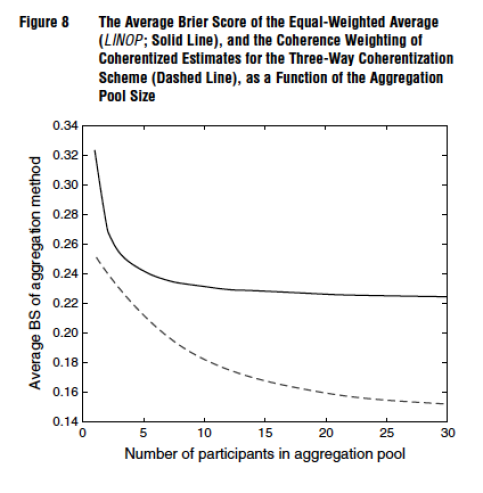
But, we also wanted to test whether the global accuracy of the entire subject sample could further be improved by weighting each subject’s contribution to a pooled estimate for a given item, A, by the degree of incoherence the subject expressed for the set of four items. That is, the less coherent one is for a given set of related items, the less they would contribute to the pooled estimate for that set. The paper describes many different instantiations of that approach, but the bottom line is that the most effective of the approaches we tested led to yet another substantial increase in accuracy for pooled judgments above and beyond that yielded by coherentization alone. There was over a 30% increase in accuracy by first coherentizing judgments and then coherence weighting subjects’ contributions to a pooled accuracy estimate.

Figure 8 from our paper, for instance, compares the average Brier score (BS) for an unweighted linear average of subjects to a coherence weighted pool for different pool sizes. As can be seen, the benefit of aggregation levels off rather quickly for the unweighted average but continues to show improvements as a function of pool size increases over a much greater range.


Screen Shot 2014-04-01 at 10.16.15 AM

When the accuracy improvement was broken down further, it translated into improvements to both calibration and discrimination. Calibration is a measure of reliability. A reliable probabilistic forecaster or judge will assign subjective probabilities that over time correspond with observed relative frequencies. So, if in 100 cases where a forecaster says he’s 80% sure the event will happen, the forecaster would be perfectly calibrated if 80 of those events occurred and 20 did not. Same would go for all the other probabilities assigned between 0 (impossibility) and 1 (necessity).

Discrimination, on the other hand, has to to with how well the forecaster or judge separates events into their correct epistemic or ontological categories. In our experiment, that involved separating statements that were true from those that were false. In a forecasting task, it might involve separating events that eventually occur from those that don’t.

One could have perfect calibration and the worse possible discrimination if one simply forecasted the base rate of an event category. For instance, in the balanced coin example, simply assigning a probability of 0.50 to each outcome ensures perfect calibration and no discrimination. In principle, one could also have perfect calibration and perfect discrimination if one were to behave like a clairvoyant — namely, by always correctly predicting outcomes with complete certainty. In principle, one could also discriminate perfectly and be completely uncalibrated. If, for instance, I forecasted like a clairvoyant except that every time I predicted occurrences with certainty the events didn’t occur and every time I predicted non-occurrences with certainty the events did occur, then I’d still have perfect discrimination because I did separate occurrences from non-occurrences. However, it’s clear that I’ve mislabeled my predictions. Such behavior is sometimes called perverse discrimination since it is odd to mix perfect discrimination with backward labelling. And sometimes it’s called diabolical discrimination (under the assumption that the forecaster or judge is trying to mislead an advisee).

Our approach benefitted both calibration and discrimination. This is important because many optimization procedures (e.g., extremizing tranformations; see, e.g., Baron et al., 2014) tinker with calibration, but leave discrimination unchanged. Yet, arguably, what matters most in many contexts involving probabilistic judgment is good discrimination — separating truth from falsity, occurrence from non-occurrence, etc.

So, we can indeed leverage the natural variation in forecasters’ logical coherence by eliciting sets of related judgments from them and then using the expressed incoherence to optimize their forecasts and optimize their forecasts’ contribution to a pool of weighted forecasts.

Oscar Wilde once said that “Consistency is the hallmark of the unimaginative.” Maybe so, but as we have learned, consistency — at least logical consistency — is also a hallmark of the accurate. That may be less quotable, but in practice it can be quite useful to know.


Credits: the opening image was found here. Apparently, it’s from punk zine called Incoherent House and was the front cover of the forth issue. Things you learn while searching for the odd image.


Gloms and Fizos Reloaded

In Gloms and Fizos, Massimo Fuggetta talks about a recent paper of his on Bayesian reasoning and reflects on the results of an earlier paper I co-authored with Gaelle Villejoubert on Bayesian reasoning and the inverse fallacy.

In the commentary, Massimo and I discuss the meaning of subjects’ violations of additivity for binary complements for which they are making posterior probability judgments — namely, the hypothetical creatures, Gloms and Fizos, who live on Planet Vuma.

Gaelle and I had found that the inverse fallacy could be used to predict whether mean additivity violations would be superadditive (adding to less than 1) or subadditive (adding to more than 1). We achieved this by structuring out stimuli so that the sums of the two relevant diagnostic probabilities for assessment pairs summed to more or less than one.

The discussion in Massimo’s Bayes blog focuses on whether researchers assessing Bayesian reasoning have an obligation to make various complementarity relations explicit for subjects. For instance, if we tell subjects that 98% of Gloms smoke cigarettes, must we also tell them that 2% don’t. Massimo seems quite convinced that doing so would eliminate additivity violations and correct their Bayesian assessments. I am less confident since I don’t think deviations from Bayes theorem are only due to people losing track of implicated information, although I agree that it would probably help, just as clarifying nested sets via natural sampling trees helps improve Bayesian judgement.

The other issue is whether there is any of sort of obligation to do so in experiments on probability judgment, and there I think the answer is clearly no. Indeed, there is no such obligation in everyday life, and the Gricean norm is to truncate redundancy. Thus, we’re not likely to say something like “I’m 95% sure I passed the exam and I’m 5% sure I didn’t.” We would either say 95% sure I passed or something like I still have a 5% doubt remaining. So the kind of truncation we used in our experiment is normative in daily life.

Reference

Villejoubert, G., & Mandel, D. R. (2002). The inverse fallacy: An account of deviations from Bayes’s theorem and the additivity principle. Memory & Cognition30, 171-178. [PDF] [Erratum]